
Introduction
La distance d’un point à un hyperplan est l’un des résultats les plus fondamentaux de la géométrie euclidienne. Derrière sa formule apparemment simple et lapidaire se cache une idée qui réapparaît dans des domaines très différents des mathématiques, notamment:
- en Optimization algorithmique, la méthode de Kaczmarz où chaque itération est exactement une projection sur un hyperplan,
- en apprentisaaage automatique, machines à vecteurs de support (SVM) où la marge d’un SVM est deux fois la distance entre les classes et l’hyperplan séparateur,
- et toujours en apprentssage automatique, l’Analyse Discriminante Linéaire (ADL) où la frontière de décision est un hyperplan, et la règle d’assignation dépend du côté où se trouve le point.
Les exemples de l’utilisation de cette notion en mathématiques sont “pléthoriques”. Dans ce billet, nous montrons comment dériver la formule de façon rigoureuse, en illustrant chaque étape géométriquement, et montrons comment elle est liée aux concepts évoqués ci-dessus. Avant de commencer, rappelons d’abord ce que c’est un hyperplan.
Rappel : l’hyperplan dans $\mathbb{R}^n$
Définition
Un hyperplan de $\mathbb{R}^n$ est un sous-espace affine de dimension $n-1$. Il est entièrement caractérisé par un vecteur normal $\mathbf{a} \in \mathbb{R}^n$ ($\mathbf{a} \neq \mathbf{0}$) et un scalaire $b \in \mathbb{R}$. C’est l’ensemble de tous les vecteurs de $\mathbb{R}^n$ dont le produit scalaire avec $\mathbf{a}$ est égal à $b$, i.e.
\[H = \bigl\{\mathbf{x} \in \mathbb{R}^n \;:\; \mathbf{a}^\top \mathbf{x} = b\bigr\}.\]Le vecteur $\mathbf{a}$ est perpendiculaire à $H$ : pour tout $\mathbf{u}, \mathbf{v} \in H$, $\mathbf{a}^\top(\mathbf{u} - \mathbf{v}) = 0$.
Autrement dit, $b$ fixe la position de l’hyperplan, tandis que les points de $H$ sont les $\mathbf{x}$ qui vérifient $\mathbf{a}^\top \mathbf{x} = b$.

Cas particuliers selon la dimension
| Dimension ambiante $n$ | $H$ = | Équation | Vecteur normal $\mathbf{a}$ |
|---|---|---|---|
| 2 | Droite | $a_1 x_1 + a_2 x_2 = b$ | $(a_1,\, a_2)^\top \in \mathbb{R}^2$ |
| 3 | Plan | $a_1 x_1 + a_2 x_2 + a_3 x_3 = b$ | $(a_1,\, a_2,\, a_3)^\top \in \mathbb{R}^3$ |
| $n$ | Hyperplan | $\mathbf{a}^\top \mathbf{x} = b$ | $(a_1,\, \ldots,\, a_n)^\top \in \mathbb{R}^n$ |
En apprentissage automatique, $n$ peut valoir des milliers (pixels d’une image, dimensions d’un embedding), mais la formule reste la même.
Cas 2D : distance d’un point à une droite
Avant de donner la formule générale, ancrons premiérement l’intuition dans le plan.
Soit la droite $H : a_1 x_1 + a_2 x_2 = b$ et un point $P = (p_1, p_2)$.
Le point $P^*$ de $H$ est plus proche de $P$ si il se trouve, en partant de $P$, dans la même direction que $\mathbf{a} = (a_1, a_2)^\top$ (le vecteur normal à la droite) :
\[P^* = P + \lambda^* \mathbf{a}, \quad \lambda^* = \frac{b - \mathbf{a}^\top P}{\|\mathbf{a}\|^2}.\]La distance est alors le déplacement effectué :
\[d(P, H) = \|P - P^*\| = |\lambda^*| \cdot \|\mathbf{a}\| = \frac{|a_1 p_1 + a_2 p_2 - b|}{\sqrt{a_1^2 + a_2^2}}.\]
Dérivation générale dans $\mathbb{R}^n$
Approche géométrique (ligne paramétrique)
Soit $H = {\mathbf{x} : \mathbf{a}^\top \mathbf{x} = b}$ et $\mathbf{p} \in \mathbb{R}^n$. Le point de $H$ le plus proche de $\mathbf{p}$ se trouve sur la droite passant par $\mathbf{p}$ et dirigée par $\mathbf{a}$ (la seule direction perpendiculaire à $H$) :
\[\mathbf{x}(\lambda) = \mathbf{p} + \lambda\,\mathbf{a}, \quad \lambda \in \mathbb{R}.\]On cherche $\lambda^$ tel que $\mathbf{x}(\lambda^) \in H$ :
\[\mathbf{a}^\top \bigl(\mathbf{p} + \lambda^* \mathbf{a}\bigr) = b \;\;\Longrightarrow\;\; \lambda^* = \frac{b - \mathbf{a}^\top \mathbf{p}}{\|\mathbf{a}\|^2}.\]Le pied de la perpendiculaire est donc :
\[\boxed{\mathbf{p}^* = \mathbf{p} - \frac{\mathbf{a}^\top \mathbf{p} - b}{\|\mathbf{a}\|^2}\,\mathbf{a},}\]et la distance est :
\[\boxed{d(\mathbf{p},\, H) = \|\mathbf{p} - \mathbf{p}^*\| = |\lambda^*|\,\|\mathbf{a}\| = \frac{|\mathbf{a}^\top \mathbf{p} - b|}{\|\mathbf{a}\|}.}\]Approche variationnelle (multiplicateurs de Lagrange)
Le même résultat s’obtient en minimisant $|\mathbf{p} - \mathbf{x}|^2$ sous la contrainte $\mathbf{a}^\top \mathbf{x} = b$. Le Lagrangien est
\[\mathcal{L}(\mathbf{x}, \mu) = \|\mathbf{p} - \mathbf{x}\|^2 + \mu\,(\mathbf{a}^\top \mathbf{x} - b).\]Les conditions du premier ordre donnent :
\[\nabla_{\mathbf{x}} \mathcal{L} = -2(\mathbf{p} - \mathbf{x}) + \mu\,\mathbf{a} = \mathbf{0} \;\;\Longrightarrow\;\; \mathbf{x}^* = \mathbf{p} - \frac{\mu}{2}\,\mathbf{a}.\]Injectant dans la contrainte :
\[\mathbf{a}^\top \mathbf{p} - \frac{\mu}{2}\|\mathbf{a}\|^2 = b \;\;\Longrightarrow\;\; \mu = \frac{2(\mathbf{a}^\top \mathbf{p} - b)}{\|\mathbf{a}\|^2},\]ce qui redonne $\mathbf{x}^* = \mathbf{p}^*$ et la même formule de distance.
Distance signée et demi-espaces
La distance signée ne prend pas la valeur absolue :
\[\delta(\mathbf{p},\, H) = \frac{\mathbf{a}^\top \mathbf{p} - b}{\|\mathbf{a}\|}.\]Son signe indique de quel côté de $H$ se trouve $\mathbf{p}$ :
| $\delta > 0$ | $\mathbf{p}$ est du côté de $+\mathbf{a}$ |
| $\delta = 0$ | $\mathbf{p} \in H$ |
| $\delta < 0$ | $\mathbf{p}$ est du côté de $-\mathbf{a}$ |
C’est exactement la quantité utilisée comme score de classification dans les modèles linéaires : $\hat{y} = \text{sign}(\mathbf{a}^\top \mathbf{p} - b)$.
Cas $\mathbb{R}^3$ : distance à un plan
Pour un plan d’équation $ax + by + cz = d$ et un point $P_0 = (x_0, y_0, z_0)$, la formule donne directement :
\[d(P_0,\, H) = \frac{|ax_0 + by_0 + cz_0 - d|}{\sqrt{a^2 + b^2 + c^2}}.\]
Exemple numérique. Plan $2x - y + 2z = 3$, point $P_0 = (1, 0, -1)$ :
\[d = \frac{|2\cdot1 - 1\cdot0 + 2\cdot(-1) - 3|}{\sqrt{4+1+4}} = \frac{|2 - 0 - 2 - 3|}{3} = \frac{3}{3} = 1.\]Cas normalisé : $|\mathbf{a}| = 1$
Si l’on normalise le vecteur normal ($\hat{\mathbf{a}} = \mathbf{a}/|\mathbf{a}|$, $\hat{b} = b/|\mathbf{a}|$), l’hyperplan s’écrit $\hat{\mathbf{a}}^\top \mathbf{x} = \hat{b}$ et les formules se simplifient :
\[d(\mathbf{p}, H) = |\hat{\mathbf{a}}^\top \mathbf{p} - \hat{b}|,\] \[\mathbf{p}^* = \mathbf{p} - (\hat{\mathbf{a}}^\top \mathbf{p} - \hat{b})\,\hat{\mathbf{a}}.\]La projection ne nécessite plus de division : on soustrait simplement la composante de $\mathbf{p}$ selon $\hat{\mathbf{a}}$ au-delà de $\hat{b}$.
Lien avec la méthode de Kaczmarz
Dans la méthode de Kaczmarz aléatoire, chaque itération résout une équation $\mathbf{a}_i^\top \mathbf{x} = b_i$ en projetant le point courant $\mathbf{x}^{(k)}$ sur l’hyperplan $H_i$ :
\[\mathbf{x}^{(k+1)} = \mathbf{x}^{(k)} - \frac{\mathbf{a}_i^\top \mathbf{x}^{(k)} - b_i}{\|\mathbf{a}_i\|^2}\,\mathbf{a}_i = P_{H_i}\!\left(\mathbf{x}^{(k)}\right).\]Le déplacement effectué a exactement la norme de la distance :
\[\|\mathbf{x}^{(k+1)} - \mathbf{x}^{(k)}\| = \frac{|\mathbf{a}_i^\top \mathbf{x}^{(k)} - b_i|}{\|\mathbf{a}_i\|} = d\!\left(\mathbf{x}^{(k)},\, H_i\right).\]La convergence est donc directement contrôlée par la rapidité avec laquelle les distances aux hyperplans diminuent.

Lien avec les SVM
Dans un Support Vector Machine linéaire, l’hyperplan séparateur est $H : \mathbf{w}^\top \mathbf{x} + w_0 = 0$ et les hyperplans de marge sont $\mathbf{w}^\top \mathbf{x} + w_0 = \pm 1$. La marge géométrique est la distance entre les deux hyperplans de marge :
\[\gamma = \frac{1}{\|\mathbf{w}\|} - \left(-\frac{1}{\|\mathbf{w}\|}\right) = \frac{2}{\|\mathbf{w}\|}.\]La distance d’un vecteur de support $\mathbf{x}_i$ à l’hyperplan séparateur est $1/|\mathbf{w}|$ — exactement notre formule avec $|\mathbf{w}^\top \mathbf{x}_i + w_0| = 1$ et $|\mathbf{a}| = |\mathbf{w}|$.
Maximiser la marge revient donc à minimiser $|\mathbf{w}|$, c’est-à-dire à maximiser la distance entre les points d’entraînement et l’hyperplan séparateur.
Lien avec l’ADL
Dans l’Analyse Discriminante Linéaire, la règle de décision pour deux classes est :
\[\hat{c}(\mathbf{x}) = \text{sign}\!\left(\mathbf{w}^\top \mathbf{x} - \theta\right),\]où $\mathbf{w} = S_W^{-1}(\mathbf{m}_1 - \mathbf{m}_2)$ et le seuil $\theta = \mathbf{w}^\top (\mathbf{m}_1 + \mathbf{m}_2)/2$.
La frontière de décision ${\mathbf{x} : \mathbf{w}^\top \mathbf{x} = \theta}$ est un hyperplan. La distance signée $\delta(\mathbf{x}) = (\mathbf{w}^\top \mathbf{x} - \theta)/|\mathbf{w}|$ donne à la fois la classe prédite (son signe) et la confiance de la prédiction (son amplitude).
Implémentation Python
import numpy as np
import matplotlib.pyplot as plt

# ── Formules de base ────────────────────────────────────────────────────────

def distance_point_hyperplan(p: np.ndarray, a: np.ndarray, b: float) -> float:
    """
    Distance de p à l'hyperplan {x : a^T x = b}.

    Paramètres
    ----------
    p : (n,) point
    a : (n,) vecteur normal (pas forcément unitaire)
    b : scalaire
    """
    return abs(a @ p - b) / np.linalg.norm(a)


def projection_sur_hyperplan(p: np.ndarray, a: np.ndarray, b: float) -> np.ndarray:
    """
    Pied de la perpendiculaire de p sur {x : a^T x = b}.
    C'est exactement l'update de Kaczmarz.
    """
    return p - (a @ p - b) / (a @ a) * a


def distance_signee(p: np.ndarray, a: np.ndarray, b: float) -> float:
    """Distance signée : positive du côté de +a."""
    return (a @ p - b) / np.linalg.norm(a)
Exemple en 2D
# Droite : 2x - y = 1  →  a = [2, -1], b = 1
a = np.array([2.0, -1.0])
b = 1.0

# Points à tester
points = {
    "P1 = (1, 0)":  np.array([1.0,  0.0]),
    "P2 = (0, 0)":  np.array([0.0,  0.0]),
    "P3 = (3, 2)":  np.array([3.0,  2.0]),
}

print(f"Droite : {a[0]:.0f}x₁ + ({a[1]:.0f})x₂ = {b:.0f}")
print(f"Norme de a : {np.linalg.norm(a):.4f}\n")

for name, p in points.items():
    d    = distance_point_hyperplan(p, a, b)
    ds   = distance_signee(p, a, b)
    pied = projection_sur_hyperplan(p, a, b)
    print(f"{name}")
    print(f"  distance          : {d:.4f}")
    print(f"  distance signée   : {ds:+.4f}")
    print(f"  pied perpendic.   : {pied}")
    print()
Résultat :
Droite : 2x₁ + (-1)x₂ = 1
Norme de a : 2.2361

P1 = (1, 0)
  distance          : 0.4472
  distance signée   : +0.4472
  pied perpendic.   : (0.6000, 0.2000)

P2 = (0, 0)
  distance          : 0.4472
  distance signée   : -0.4472
  pied perpendic.   : (0.4000, -0.2000)

P3 = (3, 2)
  distance          : 1.3416
  distance signée   : +1.3416
  pied perpendic.   : (1.8000, 2.6000)
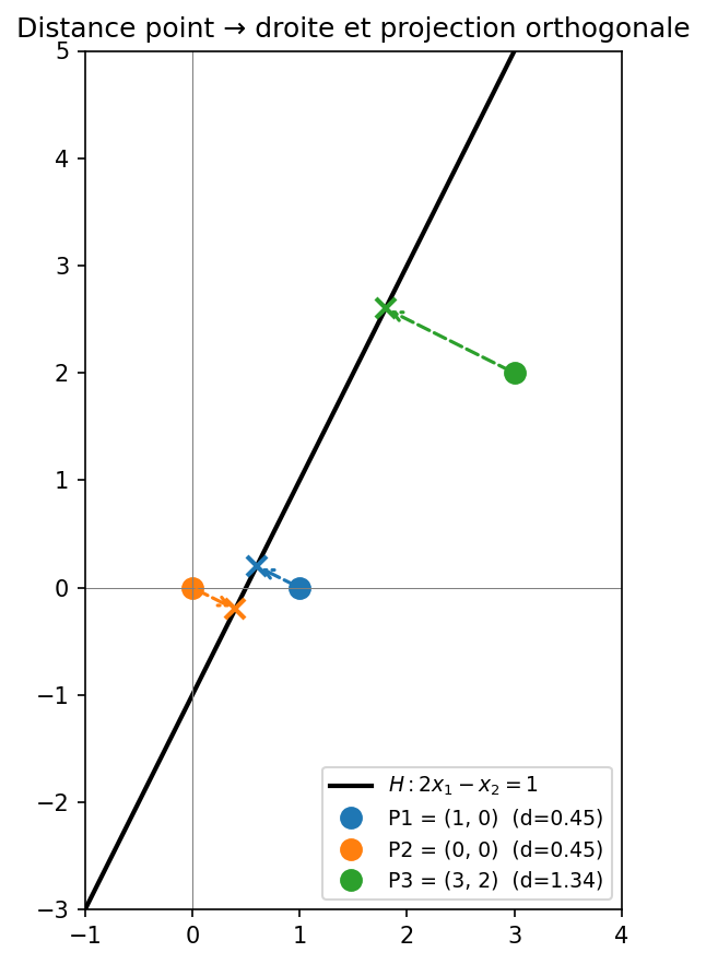
Notez que $P_1$ et $P_2$ ont la même distance à la droite ($\approx 0.4472 = 1/\sqrt{5}$) mais des signes opposés : $P_1$ est du côté de $+\mathbf{a}$ (au-dessus) et $P_2$ du côté de $-\mathbf{a}$ (en dessous). $P_3$ est presque trois fois plus loin ($\approx 3/\sqrt{5}$).
Visualisation 2D
fig, ax = plt.subplots(figsize=(7, 6))

# Tracer la droite 2x - y = 1
x_vals = np.linspace(-1, 4, 200)
y_vals = 2 * x_vals - 1
ax.plot(x_vals, y_vals, 'k-', lw=2, label=r'$H: 2x_1 - x_2 = 1$')

# Tracer les points et leur projection
colors = ['tab:blue', 'tab:orange', 'tab:green']
for (name, p), color in zip(points.items(), colors):
    pied = projection_sur_hyperplan(p, a, b)
    d    = distance_point_hyperplan(p, a, b)
    ax.plot(*p, 'o', color=color, ms=9, label=f'{name}  (d={d:.2f})')
    ax.plot(*pied, 'x', color=color, ms=9, mew=2)
    ax.annotate('', xy=pied, xytext=p,
                arrowprops=dict(arrowstyle='->', color=color,
                                lw=1.5, linestyle='dashed'))

ax.set_xlim(-1, 4); ax.set_ylim(-3, 5)
ax.set_aspect('equal')
ax.axhline(0, color='gray', lw=0.5); ax.axvline(0, color='gray', lw=0.5)
ax.legend(fontsize=9)
ax.set_title("Distance point → droite et projection orthogonale")
plt.tight_layout()
plt.show()
Généralisation $n$D — vérification
# Hyperplan en dimension 100 : a^T x = b
rng = np.random.default_rng(42)
n = 100
a_nd = rng.standard_normal(n)
b_nd = 5.0
p_nd = rng.standard_normal(n)

d_formula  = distance_point_hyperplan(p_nd, a_nd, b_nd)
pied_nd    = projection_sur_hyperplan(p_nd, a_nd, b_nd)
d_brute    = np.linalg.norm(p_nd - pied_nd)

print(f"Dimension        : {n}")
print(f"Distance formule : {d_formula:.8f}")
print(f"Distance brute   : {d_brute:.8f}")  # doit être identique
print(f"pied ∈ H ?       : {abs(a_nd @ pied_nd - b_nd):.2e}")   # ≈ 0
Résultat :
Dimension        : 100
Distance formule : 0.28027499
Distance brute   : 0.28027499
pied ∈ H ?       : 8.88e-16
Les deux distances coïncident au bit près, et la contrainte $\mathbf{a}^\top \mathbf{p}^* = b$ est satisfaite à $8.88 \times 10^{-16}$ près — l’erreur d’arrondi flottant de double précision ($\varepsilon_{\text{machine}} \approx 2.2 \times 10^{-16}$ multiplié par la taille du problème).
Récapitulatif
\[\boxed{d(\mathbf{p},\, H) = \frac{|\mathbf{a}^\top \mathbf{p} - b|}{\|\mathbf{a}\|}, \qquad \mathbf{p}^* = \mathbf{p} - \frac{\mathbf{a}^\top \mathbf{p} - b}{\|\mathbf{a}\|^2}\,\mathbf{a}.}\]| Concept | Rôle de la distance point-hyperplan |
|---|---|
| Kaczmarz | Déplacement à chaque itération = distance à $H_i$ |
| SVM | Marge = $2/|\mathbf{w}|$ = deux fois la distance |
| ADL | Distance signée = score de classification |
| Régression logistique | $\sigma(\delta)$ = probabilité de classe positive |
| Perceptron | Convergence garantie si les classes sont séparables (marge $> 0$) |
Conclusion
La formule $d = |\mathbf{a}^\top \mathbf{p} - b| / |\mathbf{a}|$ est simple à mémoriser mais ses implications sont profondes. Elle unifie la géométrie (projection sur un hyperplan), l’optimisation (condition KKT du SVM) et les solveurs itératifs (Kaczmarz). Chaque fois qu’un algorithme d’apprentissage linéaire effectue une mise à jour, il se déplace d’une quantité proportionnelle à cette distance.
Références
- Strang, G. (2016). Introduction to Linear Algebra (5th ed.), Chapter 4. Wellesley-Cambridge Press.
- Boyd, S. & Vandenberghe, L. (2004). Convex Optimization, Section 2.2. Cambridge University Press.
- Strohmer, T. & Vershynin, R. (2009). A randomized Kaczmarz algorithm with exponential convergence. Journal of Fourier Analysis and Applications, 15(2), 262–278.
- Vapnik, V. (1995). The Nature of Statistical Learning Theory. Springer.
- Bishop, C. M. (2006). Pattern Recognition and Machine Learning, Section 4.1. Springer.