
Introduction
Le problème des moindres carrés ordinaires (MCO) apparaît partout : en régression linéaire, en ADL, en traitement du signal, en reconstruction d’image. Sa formulation est simple :
\[\min_{\mathbf{w} \in \mathbb{R}^n} \;\|\mathbf{X}\mathbf{w} - \mathbf{b}\|^2, \qquad \mathbf{X} \in \mathbb{R}^{m \times n},\; \mathbf{b} \in \mathbb{R}^m.\]La solution de ce problème satisfait un système linéaire particulier appelé équation normale. Ce billet en donne deux dérivations — algébrique et géométrique — et précise quand la solution est unique.
Dérivation par la condition de gradient
Développement de la fonction coût
Notons $f(\mathbf{w}) = |\mathbf{X}\mathbf{w} - \mathbf{b}|^2$. En développant :
\[f(\mathbf{w}) = (\mathbf{X}\mathbf{w} - \mathbf{b})^\top(\mathbf{X}\mathbf{w} - \mathbf{b}) = \mathbf{w}^\top \mathbf{X}^\top \mathbf{X}\, \mathbf{w} - 2\,\mathbf{b}^\top \mathbf{X}\, \mathbf{w} + \mathbf{b}^\top \mathbf{b}.\]$f$ est une fonction quadratique convexe en $\mathbf{w}$ (puisque $\mathbf{X}^\top \mathbf{X}$ est semi-définie positive).
Condition de premier ordre
Le gradient de $f$ par rapport à $\mathbf{w}$ est :
\[\nabla_{\mathbf{w}} f(\mathbf{w}) = 2\,\mathbf{X}^\top \mathbf{X}\,\mathbf{w} - 2\,\mathbf{X}^\top \mathbf{b}.\]Un minimum est atteint là où le gradient s’annule :
\[\nabla_{\mathbf{w}} f(\mathbf{w}^*) = \mathbf{0} \;\;\Longleftrightarrow\;\; \boxed{\mathbf{X}^\top \mathbf{X}\,\mathbf{w}^* = \mathbf{X}^\top \mathbf{b}.}\]C’est l’équation normale. C’est un système $n \times n$ en $\mathbf{w}^*$, quelle que soit la taille $m$ de $\mathbf{b}$.
Pourquoi c’est bien un minimum global
$f$ est convexe (carré d’une norme), donc tout point critique est un minimum global. L’ensemble des minimiseurs est convexe ; il est réduit à un singleton si et seulement si $\mathbf{X}^\top \mathbf{X}$ est inversible, c’est-à-dire si $\mathbf{X}$ est de rang plein en colonnes ($\text{rang}(\mathbf{X}) = n$).
Interprétation géométrique
Projection orthogonale sur l’image de X
Soit $\mathcal{C}(\mathbf{X}) = {\mathbf{X}\mathbf{w} : \mathbf{w} \in \mathbb{R}^n}$ l’image (espace colonne) de $\mathbf{X}$. Le vecteur $\hat{\mathbf{b}} = \mathbf{X}\mathbf{w}^*$ est la projection orthogonale de $\mathbf{b}$ sur $\mathcal{C}(\mathbf{X})$ : c’est l’élément de $\mathcal{C}(\mathbf{X})$ le plus proche de $\mathbf{b}$.
Le résidu $\mathbf{r}^* = \mathbf{b} - \hat{\mathbf{b}} = \mathbf{b} - \mathbf{X}\mathbf{w}^*$ doit être orthogonal à $\mathcal{C}(\mathbf{X})$, c’est-à-dire perpendiculaire à chaque colonne de $\mathbf{X}$ :
\[\mathbf{X}^\top \mathbf{r}^* = \mathbf{0} \;\;\Longleftrightarrow\;\; \mathbf{X}^\top(\mathbf{b} - \mathbf{X}\mathbf{w}^*) = \mathbf{0} \;\;\Longleftrightarrow\;\; \mathbf{X}^\top \mathbf{X}\,\mathbf{w}^* = \mathbf{X}^\top \mathbf{b}.\]On retrouve l’équation normale — ici comme condition d’orthogonalité du résidu.
Schéma de la décomposition
\[\mathbf{b} = \underbrace{\mathbf{X}\mathbf{w}^*}_{\hat{\mathbf{b}}\;\in\;\mathcal{C}(\mathbf{X})} + \underbrace{(\mathbf{b} - \mathbf{X}\mathbf{w}^*)}_{\mathbf{r}^*\;\perp\;\mathcal{C}(\mathbf{X})}.\]| Composante | Appartient à | Rôle |
|---|---|---|
| $\hat{\mathbf{b}} = \mathbf{X}\mathbf{w}^*$ | $\mathcal{C}(\mathbf{X})$ | meilleure approximation de $\mathbf{b}$ par une combinaison de colonnes de $\mathbf{X}$ |
| $\mathbf{r}^* = \mathbf{b} - \hat{\mathbf{b}}$ | $\mathcal{C}(\mathbf{X})^\perp = \mathcal{N}(\mathbf{X}^\top)$ | résidu minimal irréductible |
Le théorème de Pythagore donne alors l’identité :
\[\|\mathbf{b}\|^2 = \|\hat{\mathbf{b}}\|^2 + \|\mathbf{r}^*\|^2.\]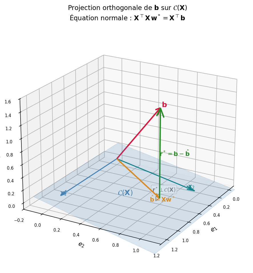
Unicité et rang
Cas rang plein en colonnes ($\text{rang}(\mathbf{X}) = n$)
Si les colonnes de $\mathbf{X}$ sont linéairement indépendantes, alors $\mathbf{X}^\top \mathbf{X}$ est symétrique définie positive (SDP) :
\[\mathbf{u}^\top (\mathbf{X}^\top \mathbf{X})\,\mathbf{u} = \|\mathbf{X}\mathbf{u}\|^2 > 0 \quad \forall\,\mathbf{u} \neq \mathbf{0}.\]L’équation normale admet alors une solution unique :
\[\mathbf{w}^* = (\mathbf{X}^\top \mathbf{X})^{-1}\,\mathbf{X}^\top \mathbf{b}.\]La matrice $(\mathbf{X}^\top \mathbf{X})^{-1}\mathbf{X}^\top$ s’appelle la pseudo-inverse de gauche de $\mathbf{X}$.
Cas rang déficient ($\text{rang}(\mathbf{X}) = r < n$)
Si $\mathbf{X}$ n’est pas de rang plein en colonnes, $\mathbf{X}^\top \mathbf{X}$ est singulière : il existe une infinité de solutions à l’équation normale (toutes donnent le même résidu minimal $|\mathbf{r}^*|$). Parmi elles, on retient souvent la solution de norme minimale :
\[\mathbf{w}^* = \mathbf{X}^{\dagger}\,\mathbf{b},\]où $\mathbf{X}^{\dagger} = \mathbf{V}\,\boldsymbol{\Sigma}^{\dagger}\,\mathbf{U}^\top$ est la pseudo-inverse de Moore-Penrose de $\mathbf{X}$ (obtenue via la décomposition en valeurs singulières $\mathbf{X} = \mathbf{U}\boldsymbol{\Sigma}\mathbf{V}^\top$ avec $\boldsymbol{\Sigma}^{\dagger}$ formée en inversant les valeurs singulières non nulles).
Tableau récapitulatif
| Système | Condition | Équation normale | Solution |
|---|---|---|---|
| Sur-déterminé ($m > n$) | $\text{rang}(\mathbf{X}) = n$ | $\mathbf{X}^\top \mathbf{X}$ SDP | unique : $(\mathbf{X}^\top \mathbf{X})^{-1}\mathbf{X}^\top \mathbf{b}$ |
| Carré ($m = n$) | $\mathbf{X}$ inversible | $\mathbf{X}^\top \mathbf{X}$ SDP | unique : $\mathbf{X}^{-1}\mathbf{b}$ |
| Sous-déterminé ($m < n$) | $\text{rang}(\mathbf{X}) = m$ | $\mathbf{X}^\top \mathbf{X}$ singulière | $\infty$ solutions ; norme min : $\mathbf{X}^{\dagger}\mathbf{b}$ |
| Rang déficient | $\text{rang}(\mathbf{X}) = r < \min(m,n)$ | $\mathbf{X}^\top \mathbf{X}$ singulière | $\infty$ solutions ; norme min : $\mathbf{X}^{\dagger}\mathbf{b}$ |
Cas ADL-MCO sur Olivetti Faces
Dans notre application, $\mathbf{X}_c \in \mathbb{R}^{300 \times 4096}$ ($N=300 \ll d=4096$). On est dans le cas sous-déterminé : le système $\mathbf{X}_c \mathbf{w} = \mathbf{t}$ est toujours consistant (il existe des $\mathbf{w}$ qui l’annulent exactement), mais $\mathbf{X}_c^\top \mathbf{X}_c$ est singulière. La solution de norme minimale $\mathbf{w}^* = \mathbf{X}_c^{\dagger}\mathbf{t}$ est celle choisie par LSQR et Kaczmarz étendu (REK) — sans jamais former $\mathbf{X}_c^\top \mathbf{X}_c \in \mathbb{R}^{4096 \times 4096}$.
Conclusion
L’équation normale $\mathbf{X}^\top \mathbf{X}\,\mathbf{w} = \mathbf{X}^\top \mathbf{b}$ est le cœur du problème MCO. Elle admet deux lectures complémentaires :
- Algébrique : annulation du gradient de la fonction coût quadratique.
- Géométrique : orthogonalité du résidu à l’image de $\mathbf{X}$, autrement dit projection de $\mathbf{b}$ sur $\mathcal{C}(\mathbf{X})$.
L’unicité de la solution dépend entièrement du rang de $\mathbf{X}$ : rang plein en colonnes si et seulement $\mathbf{X}^\top \mathbf{X}$ inversible si, et seulement solution unique. En cas de rang déficient, la pseudo-inverse de Moore-Penrose sélectionne la solution de norme minimale — celle que retournent LSQR et les méthodes de Kaczmarz.
Références
- Strang, G. (2016). Introduction to Linear Algebra (5th ed.). Wellesley-Cambridge Press.
- Trefethen, L. N. & Bau, D. (1997). Numerical Linear Algebra. SIAM.
- Björck, Å. (1996). Numerical Methods for Least Squares Problems. SIAM.